Whenever I go to a new place and have to choose a place to eat, or whenever I am looking for new earphones, I end up stuck in the same dilemma : should i choose the option with the most reviews ? Or the one with the best rating ?
Let’s imagine you are in a new city and look for a place to have dinner tonight. You quickly look up on the web and come up with two options:
- Option A: A hidden gem sushi spot with a 5.0-star rating… but only 3 reviews
- Option B: A popular local chain with a 4.3-star rating… but 2,500 reviews
Which one would you choose ?
If we were presented with average ratings only, we would choose A. Fortunately (or not), ratings are often coming with number of reviews, and this is where our brains get confused. Your human intuition says: “Wait, 3 reviews could just be the owner’s mom and two friends. 4.3 stars across 2,500 people is social validation.”
We make choices everyday, and most of the choices we make can be summarized as a tension between two different forces: exploration and exploitation.
- “Exploration” is about taking risks and exploring less well-known options.
- “Exploitation” is about following the general consensus or options which seem safer.
This trade-off is everywhere:
- traders managing a portfolio and trying to maximize their returns.
- Websites trying to choose which products they should display to their users to maximize conversion.
- Netflix deciding which movies you will most likely watch.
So going back to our restaurants, and the critical question: how do we choose ? Or if we rephrase: how do we make the best decision ?
In bayesian statistics, the best choice is often linked to something we call minimizing regret. We will come back to this notion later. But for now, we would like a simple solution to balance reviews and ratings to make the best choice that takes into account both factors.
Why averages lie
There is a simple formula to balance ratings and reviews, used by the famous IMDB database (used to rank movies).
$$ \text{Bayesian Rating} = \frac{(R \times v) + (C \times m)}{v + m} $$
Where: - $R$ = The raw average rating of the specific item/restaurant. - $v$ = The number of reviews it has. - $m$ = A threshold number of reviews (e.g., 50 reviews to be taken seriously). - $C$ = The average rating across the entire website (e.g., 4.0 stars).
When $v$ is tiny (e.g., 2 reviews): $m$ dominates the denominator, and $C \times m$ dominates the numerator. The rating gets dragged straight toward the platform average ($C$).When $v$ is massive (e.g., 5,000 reviews): $v$ completely overpowers $m$, the $C \times m$ term becomes negligible, and the score simplifies to $R$ (the raw average).
However, while simple, this solution has several drawbacks:
-
This formula assumes ratings follow a normal distribution, which is not the case. In most cases, ratings are either binary (click/don’t click, like/dislike), or multinomial (rating from 1-5, poor/average/good/excellent, etc). You cannot give a 3.542525 rating to a restaurant. So this formula unfortunately does not work in our case.
-
The other problem is that averages can reflect very different realities. Think about:
- A restaurant with twenty 5-star reviews and twenty 1-star reviews averages out to 3.0 stars.
- A restaurant with forty 3-star reviews also averages out to 3.0 stars.
Both restaurants show an average rating of 3.0, but to a human consumer they are wildly different. The first is a highly controversial, risky gamble; the second is the definition of an “average” restaurant, on which people seem to agree.
-
Finally, in the real world of e-commerce and Google reviews, people rarely leave 3-star reviews. They usually leave a 5-star review if they are thrilled, or a 1-star review if their order was broken or late. This creates a bimodal (camel-like) distribution.
Thinking “Bayesian”
To model this problem, we can use a Bayesian framework. Bayesian statistics are actually very close to how the human brain learns and takes decisions. A child quickly learns that putting its hand in the fire will burn. It does not need to repeat the experiment 1000 times. Let’s describe this situation in a Bayesian framework, in which we want to learn the probability that i harm myself given fire:
- Prior: there is a flame, but i don’t know if it hurts or not.
- Observation: i put my hand in the fire, it burns
- Posterior: i update my knowledge. I know the probability i get burned by a flame is stronger now.
In our restaurant case, the prior would be: “They usually leave a 5-star review if they are thrilled, or a 1-star review if their order was broken or late”. We then gather data (also called evidence) to update our prior belief. Either it strengethens our belief, or it goes against it. We end up with a posterior distribution that shows the final prior + data update.
The naive approach : computing means
The naive approach before doing anything bayesian is to compute the means of our ratings:
obs_counts_A = np.array([0, 0, 0, 0, 3])
obs_counts_B = np.array([10, 2, 8, 30, 50])
star_values = np.array([1, 2, 3, 4, 5])

avg_rating_A = np.dot(obs_counts_A, star_values) / obs_counts_A.sum()
avg_rating_B = np.dot(obs_counts_B, star_values) / obs_counts_B.sum()
This yields: - $\text{Avg rating A}=5$ - $\text{Avg rating B}=4.08 $
The Bayesian approach: computing distributions
There is a nice property about Bayesian statistics which is conjugate priors. Conjugate priors are distributions which allow to compute posteriors without any sampling. In our case, using a Dirichlet prior and a Multinomial likelihood allows us to get a Dirichlet posterior from a direct formula:
$$\text{posterior} = Dirichlet(\alpha_{prior} + \text{observed counts}) $$
import scipy
import numpy as np

# ratings
obs_counts_A = np.array([0, 0, 0, 0, 3])
obs_counts_B = np.array([10, 2, 8, 30, 50])

# prior knowledge: we assume all ratings have the same probability
alpha_prior_a = [1,1,1,1,1]
alpha_prior_b = [1,1,1,1,1]

# Compute samples
d_a = scipy.stats.dirichlet(alpha=alpha_prior_a+obs_counts_A)
d_b = scipy.stats.dirichlet(alpha=alpha_prior_b+obs_counts_B)
s_a = d_a.rvs(1000)
s_b = d_b.rvs(1000)

# Compute expected average score
star_values = np.array([1, 2, 3, 4, 5])
expected_scores_A = np.dot(s_a, star_values)
expected_scores_B = np.dot(s_b, star_values)
As simple as that.
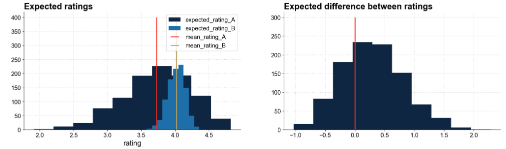
What we see here is that the expected score distribution for B is narrower compared to A. This is expected since A has more reviews and “converges” to a narrower distribution. If we now take the means of both distributions, we see A now has a lower mean vs B, compared to the naive computation we did before.
The right-hand side plot also shows the distribution of differences between the expected scores of A and B. It answers the question “how better is B vs A, probabilistically speaking”. As shown, the distribution is shifted towards the right and not centered on 0. We can conclude that B is indeed better than A.
Before we dive into a solution on how to choose the best restaurant, let’s take a moment to talk about time decay.
Time decay
In our current setup, an observation from three years ago carries the exact same weight as an observation from yesterday. But in the real world of e-commerce and restaurant reviews, data rots. A restaurant might have hired a terrible new chef last month.
If you don’t account for time, old data creates massive inertia. A product with 5,000 old 5-star reviews will completely drown out a recent wave of 1-star reviews.
To fix this, we apply an exponential decay factor ($\gamma$) to our historical data. The parameter $\gamma$ (gamma) lives between 0 and 1 (usually something like $0.95$ or $0.99$ per week).Instead of just adding up all reviews historically, you multiply your existing counts by $\gamma$ every time a new time step occurs before adding the new reviews.Over time, your posterior alpha parameters look like this:
$$\alpha_{\text{t}} = \alpha_{\text{prior}} + \sum_{i=1}^{t} \gamma^{t-i} \cdot \text{Observed Counts}_i$$
So, which one do i choose ?
The first, quick and dirty answer would be: “it depends”. You like risk and are open to having a bad dinner experience ? Take option A. You are going on a date and cannot afford a bad experience ? Take option B.
The other answer is to take a lower percentile of the posterior distribution instead of the mean. This answers the question: “In a pessimistic but plausible scenario, how good is this restaurant?”
Restaurant A might have a higher mean (say 4.1), but its 10th percentile could be as low as 3.6 — reflecting the massive uncertainty from only 3 reviews. Restaurant B’s 10th percentile sits comfortably at 3.9. If you want to minimize your downside risk, the choice becomes obvious.

Though A and B have close expected score means in this case, the 10th percentile of B’s expected scores is clearly lower compared to A. The spread between the 10th percentile and the mean is a good indication of the uncertainty
This is essentially what risk-averse decision-making looks like in Bayesian terms: you’re not asking “which is probably better on average?” but “which one am I least likely to regret?”
Going further: how websites make choices
While you are doing bayesian experiments when choosing a restaurant, the platform is also doing one on you ! Indeed, restaurants, or products on an e-commerce website, are not presented at random.
Amazon and Google know that if they only show you the bestsellers with the most reviews (pure exploitation), the platform will stagnate, and converge to a point where a small portion of available products get displayed and sold. New and potentially amazing products would never get discovered.
A platform like Netflix does exactly the same: it runs an algorithm called Multi-Arm Bandits (MAB) on its search results page. MAB allow to balance exploration and exploitation, to minimize total regret. In Netflix’s case, regret is the user bounce rate (meaning not selecting a displayed video). In a perfectly designed home page, you would watch all movies that are presented to you.
So how does a home page using MAB works ? It balances the results in the following fashion:
- X% of the results it shows you are the proven bestsellers to ensure you actually buy something today.
- (100-X)% of the results are “exploratory” slots where the algorithm takes a risk and injects a brand-new product with only 2 reviews onto the first page.
The X is exactly why we need this experiment. A high X means you favor exploitation (bestsellers). A low X favors discovery and exploration.
The name “Multi-Arm Bandit” is directly coming from casinos and slot machines. When playing slot machines, the player wants to choose the machine with the highest reward, with as little trials as possible. Comparison with e-commerce or Netflix is immediate: they want to know which options will lead you to purchase or to watch and maximize revenue or time spent on the platform
By clicking on or ignoring a recommendation from the website, you provide the data that the website’s bandit needs to update its algorithm. You are the data point in their experiment, using your own internal experiment to buy a product!
But how exactly does the bandit decide when to explore and when to exploit? The mechanism is surprisingly close to what we just built.
In the restaurant rating problem, we used a 5-star rating distribution (The Dirichlet-Multinomial). In the Netflix case, we can simplify the 5-star scale to a simpler boolean distribution: the Beta distribution, when there are only two outcomes (click or no click, buy or don’t buy, etc). And that Beta posterior is the engine inside algorithms like Thompson Sampling, which platforms use to dynamically allocate traffic between options.
In the next sections, we’ll look at how this works in practice, and compare it to the more traditional approaches used in A/B testing.
Frequentist, Bayesian A/B testing and MAB
So let’s imagine we now work for a company running an e-commerce business, and we are presented with two options for the product listing page. The goal is to maximize user conversion, ie users clicking on presented products. We need to allocate traffic for 100000 users daily.
In real life, we know absoluterly nothing about conversion rates, but just like slot machines, we want to find as early as possible the version that maximizes conversion: each missed sale is lost money. For the sake of the demo here, we will generate data with respectively 4% and 6% conversion rates.
This is a classical A/B test experiment, for which we basically have 3 options:
- Fixed 50/50 split, compute z-test after collecting data for the 100000 users
- Fixed 50/50 split, compute $P(B > A)$. When $P(B > A)$ exceeds your threshold (e.g., 95%). stop.
- Initial 50/50 split, update posterior, sample, and pick the best option at each iteration. Traffic split will shift.
Let’s design three samplers for that, and run our little experiment.
true_rates = {"A": 0.04, "B": 0.06} # Unknown in real life !
n_visitors = 10_000
best_rate = max(true_rates.values())

def simulate_click(arm):
    return np.random.binomial(1, true_rates[arm])  # returns 0 or 1

class FrequentistStrategy:
    def __init__(self):
        self.results = {
            "A": [],
            "B": []
        }
        self.regret = []
        self.allocations = []

    def sample(self, i):
        arm = "A" if i % 2 == 0 else "B"
        self.allocations.append(arm)
        click = simulate_click(arm)
        self.results[arm].append(click)
        self.regret.append(best_rate-true_rates[arm])


class BayesianStrategy:
    def __init__(self):
        self.results = {
            "A": [],
            "B": []
        }
        self.successes = {"A": 0, "B": 0}
        self.trials = {"A": 0, "B": 0}
        self.regret = []
        self.allocations = []
        self.p_b_beats_a = []

    def sample(self, i):
        arm = "A" if i % 2 == 0 else "B"
        click = simulate_click(arm)
        self.successes[arm] += click
        self.trials[arm] += 1
        self.allocations.append(arm)
        self.results[arm].append(click)
        self.regret.append(best_rate-true_rates[arm])

        samples_a = scipy.stats.beta.rvs(
            1 + self.successes['A'],
            1 + self.trials['A'] - self.successes['A'],
            size=1000)

        samples_b = scipy.stats.beta.rvs(
            1 + self.successes['B'],
            1 + self.trials['B'] - self.successes['B'],
            size=1000)
        self.p_b_beats_a.append((samples_b > samples_a).mean())


class ThompsonStrategy:
    def __init__(self):
        self.results = {
            "A": [],
            "B": []
        }
        self.priors = {
            "A": {"alpha": 1, "beta": 1},
            "B": {"alpha": 1, "beta": 1}
        }
        self.successes = {"A": 0, "B": 0}
        self.trials = {"A": 0, "B": 0}
        self.regret = []
        self.allocations = []

    def sample(self, i):
        sample_a = scipy.stats.beta.rvs(
            1 + self.successes['A'],
            1 + self.trials['A'] - self.successes['A'],
            size=1)
        sample_b = scipy.stats.beta.rvs(
            1 + self.successes['B'],
            1 + self.trials['B'] - self.successes['B'],
            size=1)
        arm = "A" if sample_a > sample_b else "B"
        click = simulate_click(arm)
        self.successes[arm] += click
        self.trials[arm] += 1
        self.allocations.append(arm)
        self.results[arm].append(click)
        self.regret.append(best_rate-true_rates[arm])


freq_sampler = FrequentistStrategy()
bayesian_sampler = BayesianStrategy()
thompson_sampler = ThompsonStrategy()


for i in range(n_visitors):

    freq_sampler.sample(i)
    bayesian_sampler.sample(i)
    thompson_sampler.sample(i)
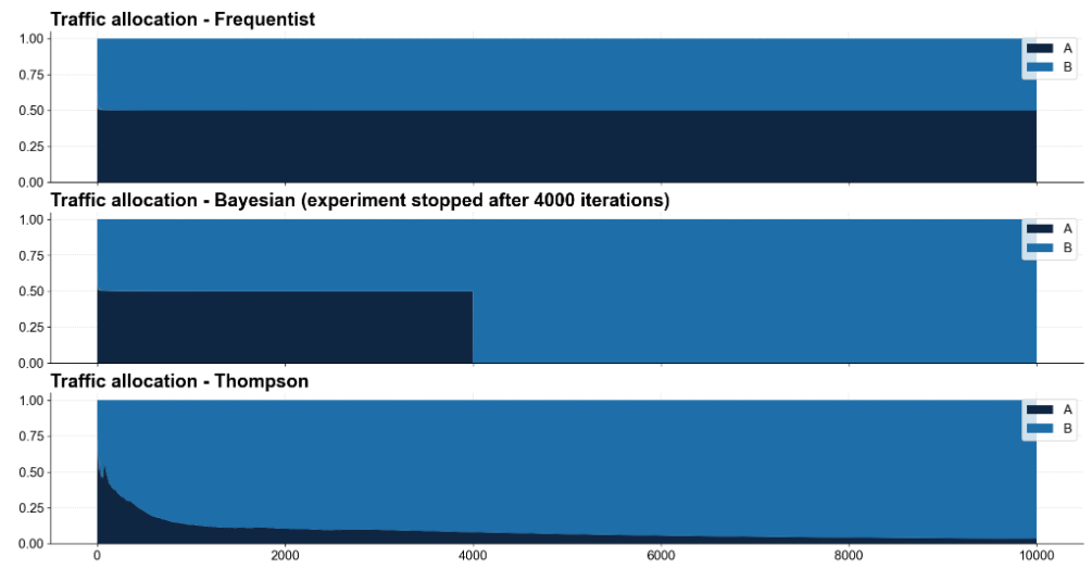
The FrequentistSampler is the simplest one: it always assigns 50% of the traffic to option A, and 50% to option B. We have to wait until the end to know if groups are statistically different.
The BayesianSampler does the same allocation strategy BUT it computes at every step the probability that $B$ is truly better than $A$:

It quickly converges to 1 after 4000 iterations, meaning we could stop the experiment earlier. We cannot do that with the frequentist sampler: running a Z-test after each iteration increases the risks of seeing a false positive p-value. This is one of the main drawbacks of running frequentist tests: peeking at values during the test is forbidden, otherwise statistical tests might incorrectly reject the null hypothesis.
Finally, the ThompsonSampler adopts another strategy: it explores arms/options at the early stages, and quickly learns which option is the best. Looking at the cumulative regrets for all three strategies, we see that both FrequentistSampler and BayesianSampler overlap (since their allocation strategy is the same), and that ThompsonSampler quickly plateaus, meaning the regret does not increase anymore: ThompsonSampler has learned which option was the best.

Now if we look at the traffic allocation, we will clearly see how ThompsonSampler adapts its allocation strategy. We can also see what the BayesianSampler allocation would look like if we decided to stop the experiment after 4000 iterations (when $P(B<A)$ gets close to 1)
In a nutshell, here is a summary of the three methods:
| Approach | Description | Pros | Cons |
|---|---|---|---|
| Frequentist | Fixed 50/50 split, chi-squared or z-test, wait for p < 0.05. | Simple & well-known |
|
| Bayesian A/B test | Fixed 50/50 split, Beta posteriors, compute $P(B > A)$ at any point. |
|
Knowing when to stop |
| MAB | Dynamic allocation. Each round: sample from each variant’s Beta posterior, send traffic to whichever sampled higher. | As evidence accumulates: allocation shifts toward the winner | If underlying conversion rates for A and B are close, it can choose the wrong arm early |
Conclusion
From picking a restaurant to ranking products to running A/B tests to optimizing ad campaigns — it’s all Bayesian updating and the explore/exploit tradeoff.
So next time you’re standing on that street corner choosing a restaurant, you can tell your date : “Let me just run a quick Thompson sampling in my head before I decide”.
And please do let me know if this seduction technique works ;)
The difference between A/B testing and bandits isn’t the math, it’s what you optimize for: knowledge (exploration) or revenue (exploitation).
| Feature | Bayesian A/B Testing | Bayesian Multi-Arm Bandits |
|---|---|---|
| Traffic Split | Static (Fixed 50/50 throughout) | Dynamic (Adjusts based on performance) |
| Primary Goal | Finding the absolute truth/statistical certainty. | Maximizing conversions/revenue during the test. |
| Best Used For | Long-term strategic changes (e.g., redesigns, pricing models, branding). | Short-lived opportunities (e.g., news headlines, holiday ad campaigns, flash sales). |
| Sample Size | Often requires larger overall sample sizes to reach definitive conclusions. | Saves sample size by starving losing variations early. |