Let’s go back in time and see if we can end up with a different winner for the NBA 2019 title. How ?By using Bayesian simulations.

[This article was inspired by the work of Baio and Blangiardo (2010), Daniel Weitzenfeld’s great blog article, and Peadar Coyle’s *tutorial *on Hierarchical models.]
Introduction
Bayesian simulation relies heavily on statistical distributions to model outcomes and therefore serves as a tool for simulating scenarios. At its base lies Bayes’ theorem. Bayes’ formula contains 4 parts : the posterior, the prior, the likelihood, and the evidence. Going into the details of each of it is not the goal of this article, but just keep in mind that the process is the following : starting from a prior distribution which we think models the phenomenon we observe (think “toss a coin”), we gather data (the likelihood), and use this data to update our prior belief about our distribution and turn it into a posterior distribution.
Why is it appropriate for our case study ?
We want to estimate the strength of each team and be able to run simulations with these informations. The only information we have access to are the scores. We do not know the strength of each team beforehand (ie we say that this is a latent variable), but we know that if we have access to a team’s strength, we can pick another team and compare their strengths to see which one will win the confrontation. Last but not least, to estimate a team’s strength, we use scores, but this data can be noisy : it might not reveal the true strength of a team at a given moment, for example if its best player was injured, etc. Hopefully, Bayes comes to our rescue because Bayesian simulations allow us to:
- model latent variables given observations
- get distributions instead of point estimates for our variables, which is good if we want to take uncertainty into account
- sample from the obtained distributions (the generative model for our phenomenon) to simulate new observations
Going back in time
Now you’re convinced that a Bayesian simulation is what we need, we are going to take a step back in time and go back to April 12th, 2019. The regular season has just ended, and playoffs will start tomorrow. Each of the 30 NBA league teams have played 82 games. This data is what we need to build our Bayesian model in order to estimate each teams’ strengths.
Once we have each team’s strengths, we will simulate several playoffs scenarios and see which team wins in the end. Ready ?
Collecting the data
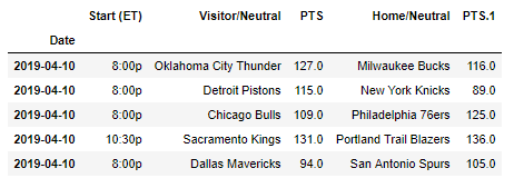
The data was collected from the website https://www.basketball-reference.com, where you can get all the results of the 2019 season. We store everything inside a DataFrame and make sure we only keep the regular season’s games.
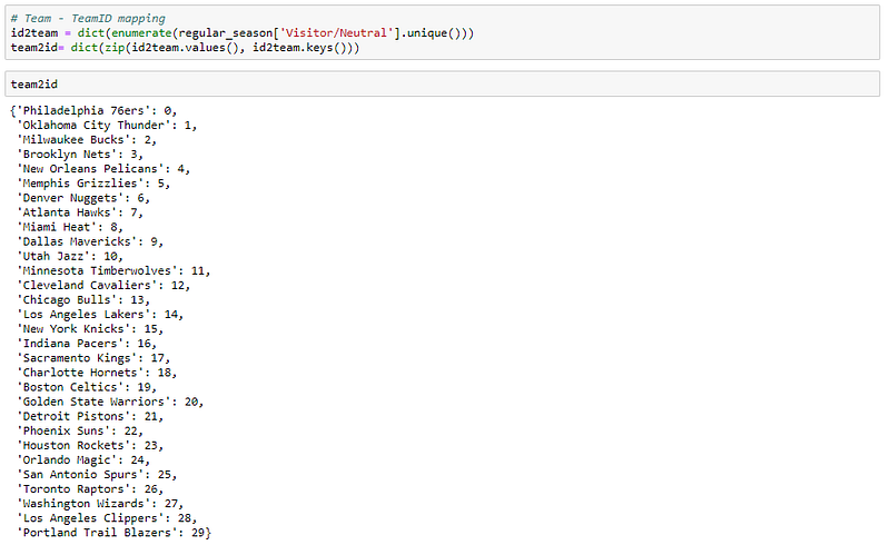
We then map all of our teams to a unique id :
Preparing the model
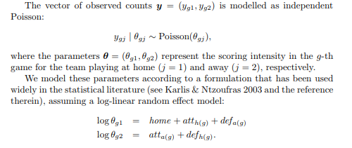
The model is taken from Baio and Blangiardo (paper here). It is a simple log-linear model which allows to model any game opposing two teams. Here is how it works :
- For a given game, the scores can be modelled as (y1, y2) where each yi are taken from a Poisson distribution (reminder : a Poisson distribution is a discrete value distribution used to model count events during a fixed period of time).
- Each Poisson distribution for a given yi is parametrized by a rate ϴ(i) which represents the combination of the team’s attack strength and its opponent’s defense strength.
- As a consequence, if a team A has a strong attack and its opponent B a weak defense, ϴ(A) will be large, and therefore the samples obtained from the Poisson(ϴ(A)) distribution will be large too. Thus increasing the number of points scored by team A.
- To ensure ϴ is positive, we model it as a log linear equation.
And voilà !
Choosing priors
Now we have our model to link the observed scores with Poisson and therefore ϴ, we have to model the att and def parts of the equation. In our case, we believe that the attack strength att and defense strength def should be, on average, zero. Strong teams will have values above zero, weak teams below zero. Furthermore, we have no a priori belief on att and def, so we will use a Normal prior with a mean taken from a hyper-prior allowing for values close to zero (in cour case, a highly skewed Normal around zero). For the standard deviation of the Normal priors, we will use a hyper-prior which allows for small positive values of std dev (in our case, it’s a Gamma distribution).
Here is the model :
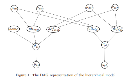
The circles at the top, mu and tau, are our hyper-priors. This model is called a Hierarchical Bayesian Model.
And here is the code:
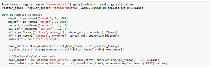
Notice how we’ve ignored the “home” parameter in the equation and how we’ve added the “intercept” parameter.
Run the Monte-Carlo
PyMC3 uses Monte-Carlo Markov Chain for finding the right distributions for our model. Explaining MCMC is beyond the scope of this article, but I can recommend this excellent article by Thomas Wiecki (one of the main contributors of PyMC3) if you want to know more about it.
After running the MCMC sampler, we visually inspect our distributions. If the distributions of a given variable overlap, this is good sign and shows the MCMC has converged to a stable solution. Another way of checking convergence is by looking at the traces of the right hand side of the graph and see if the traces look like white noise (ie no change in trend, no change in amplitude).
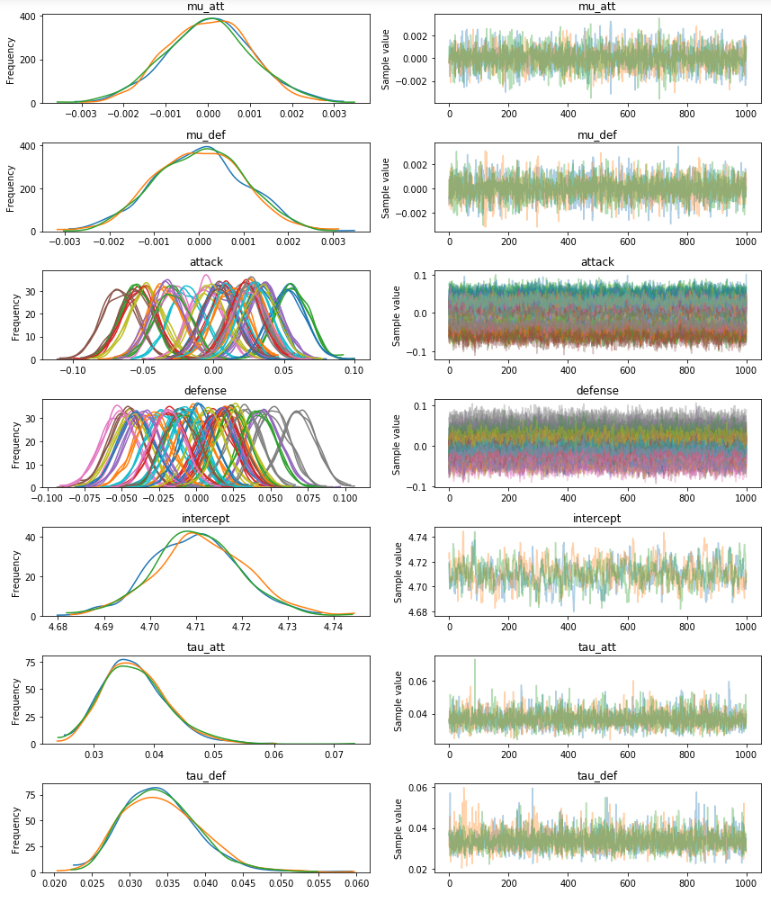
See how the distributions for each variable overlap ? Of course there are other ways of checking convergence, one of them being the R-hat statistic. You can see it by plotting a forestplot of a given parameter:
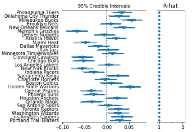
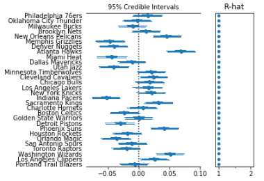
The R-hat is 1 in all cases, that’s a sign our algorithm has converged. Based on these graphs, we can see which teams have the best attacks and best defenses (Careful: signs are reversed for defense ! A good defense has a negative score !):
- Attacks : Milwaukee, Golden State, New Orleans
- Defenses : Indiana, Memphis, Miami
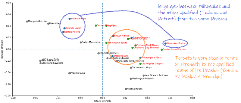
Let’s wrap this up on a scatterplot (for better readability, I reversed the sign of defenses : good defense = positive score):
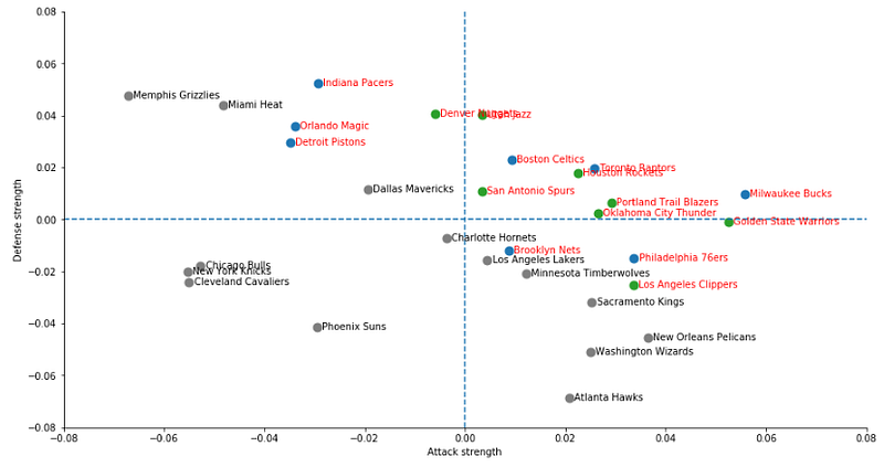
Red labels : the teams which qualified for playoffs. Blue dots: Western conference Green dots: Eastern conference.
Intermediate conclusion : Based on the above graph, Milwaukee seems to have the strongest attack, altogether with an “average” defense. The Toronto Raptors have a significantly lower attack strenght, with a slightly higher defense strength.
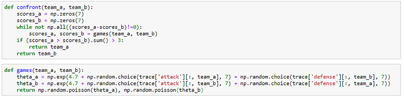
Now we have an attack and a defense strength distribution for each team, we can simulate games ! If I sample from those distributions, I can compute
- score_A = sample_Poisson(sample_attack(A)+sample_defense(B)+intercept_mean)
- score_B = sample_Poisson(sample_attack(B)+sample_defense(A)+intercept_mean)
Comparing score_A vs score_B allows me to get the winner !
Here is the code :
Simulating Playoffs
Based of the regular season results (remember, we are currently on April 12th !), here’s what I see:
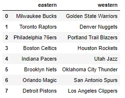
I know, based on these rankings, that the 1st round of playoffs will be :
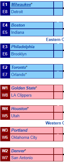
Here is the process of one scenario:
- For each game in the 1st round configuration, we calculate 7x2 samples for each team (7 attacks, 7 defense) to know the winner across the 7 games (no ties are allowed). We keep the 8 winners.
- We then have a Conference Semifinals configuration. (8 teams remaining)
- For each game in the Conference Semifinals, we calculate 7x2 samples for each teams (7 attacks, 7 defense) to know the winner across the 7 games (no ties are allowed). We keep the 4 winners.
- We then have a Conference Finals configuration. (4 teams remaining)
- For each game in the Conference Finals, we calculate 7x2 samples for each teams (7 attacks, 7 defense) to know the winner across the 7 games (no ties are allowed). We keep the 2 winners.
- We then have a NBA Finals configuration with two teams.
- We again calculate our samples across 7 games to get the final winner
Results
And here is what we get if we run 1000 playoffs simulations :
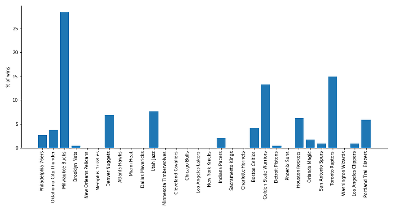
Milwaukee wins the title in more than 25% of the cases ! In more than 15% of the times, Toronto would win. Golden Stats comes 3rd with a frequence of wins around 15%
Explanation
The data is slightly biased during the regular season due to the imbalance between Divisions. As a consequence, it is likely that Milwaukee comes from a “weak” Division, therefore getting overestimated attack and defense strengths. Similarly, Toronto’s division is much more balanced in terms of strengths, thus getting underestimated. Let’s compare Milwaukee’s Division with Toronto’s :
Conclusion
I hope you had fun revisiting the NBA 2019 Playoffs. Feel free to share any thoughts on the results, and how you would incorporate a “Division” effect in our model to account for the unequal Division levels !