In this article, we will forecast the number of FHV (For Hire Vehicles, like Uber) in New York using LSTMs. We will learn how to add confidence intervals to our forecasts using Monte-Carlo dropout.

Introduction
LSTM (Long Short-Term Memory) is a type a type of recurrent neural network (RNN) architecture, and was proposed in 1997 by Sepp Hochreiter and Jürgen Schmidhuber. RNNs are Deep neural networks specially designed to handle sequential data via recurrence mechanisms. They behave in an autoregressive manner, as they keep track of the past via internal states (hence the “memory” part). They have been used extensively for speech recognition, machine translation, speech synthesis, etc. But what are LSTMs worth when used on time-series ? Well, they can prove to be very useful to model non-linear relationships, assuming the size of the data available is large enough..
The Uber use case: Bayesian forecasting
When looking for papers implementing time series forecasting with LSTMs, I found a paper written by Uber in 2017, “Deep and Confident Prediction for Time Series at Uber”. The basic question behind this paper is : how confident can we be (ie how can we quantify uncertainty) making predictions with LSTMs ?
The approach developped by Uber is a mixture of an encoder-decoder (used as an autoencoder) and a fully connected feed-forward network, used to predict the number of trips in a city based on previous data, or to detect anomalies in real time.
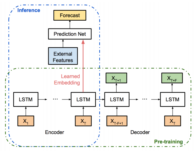
The Uber paper is one of the first to use a Bayesian approach for time series forecasting. If you want to know more about Bayesian neural networks and Bayesian inference, you can look at the following links:
- Making your Neural Network Say I Don’t Know
- Dropout as a Bayesian Approximation
- Deep Bayesian Neural Networks
- Bayesian Methods for Hackers, Cameron Davidson-Pilon
Bayesian Neural Networks
To put Bayesian neural networks in a nutshell, BNNs estimate a probability distribution over each weight, whereas classical Neural networks try to find the optimal value for each weight. When you hear “Bayesian”, think “probability distribution”.
— But what’s the link between forecasting uncertainty and Bayesian networks ?
Imagine two weather experts, Bob and Alice. You both know they are quite good at predicting weather temperatures, but sometimes they get it wrong too. You ask them what will the temperature be tomorrow at 8am so you can know if you need to put your coat on or not. Bob says : “It will be 15.6°C”. Alice says : “I’m 95 percent sure that the temperature will be between 16 and 18°C”. Although they do not seem to agree, who would you trust ?
Personally, I would trust Alice for two reasons:
- She gave me a confidence interval. I feel more reassured when someone is able to tell me something and how much he/she is confident with this information.
- I do not really care about the exact temperature, because a 1°C difference in temperature will not influence my decision to put on my coat.
However, had Alice told me “I’m 95 percent sure that the temperature will be between 0°C and 18°C”, I would have said that although she gave me a confidence level, the interval is too large to be informative…
Uncertainty under the BNN framework
We usually separate uncertainty in 3 categories : model uncertainty, inherent noise, and model misspecification. The first two are the most famous and are usually referred to as epistemic and aleatoric uncertainty. Model (or epistemic) uncertainty is the uncertainty about our model parameters. The more data you have, the more you can explain (ie “reduce”) this uncertainty. Noise (or aleatoric) uncertainty refers to the noise in the observations. If the noise uncertainty is constant for all samples, we call that homoscedastic aleatoric uncertainty. Otherwise, if some samples are more incertain than others, we will use the term heteroscedastic aleatoric. Noise uncertainty cannot be reduced with more data.
In the Uber paper, a third uncertainty is used : model misspecification. This uncertainty aims to “ capture the uncertainty when predicting unseen samples with very different patterns from the training data set”.
— Now why distinguish all of these uncertainties ?
Well, precisely because some can be combated with more data (model/epistemic), and some cannot. Some researchers therefore argue that it is more relevant to focus on aleatoric uncertainty given it cannot be reduced even with more data (Kendall & Gal, 2017)
In this article, we will only focus on the model uncertainty, to keep it simple. Uber uses different algorithms to evaluate the two other uncertainty types, but investigating them is beyond the scope of this article.
Getting and Preparing the data
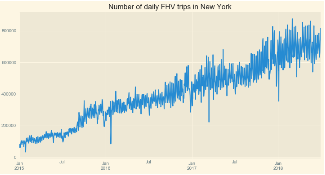
The authors in the paper use 4 years of data over 8 cities in the US to train their model. 3 years are used for training and 1 year for testing. Unfortunately, Uber hasn’t released this data yet, but in order to reproduce results from their paper, we will use data available on the New York Open data portal. We selected three years of data, spanning from early 2015 to mid 2018. Data was resampled with a daily basis. Here is what the full data looks like
Stationarity
We can notice a couple of things which you should be familiar with if you’re used to analyzing time-series:
- We observe a clear upwards trend
- Mean and variance increase through time
- We also observe spikes which may be caused by external events (holidays and weather ?)
The first two bullet points are a sign that our series is clearly not stationary. The latter shows that we might need to incorporate external data to our series. Stationarity could be checked with an Augmented Dickey-Fuller test or a KPSS test. So should we carry out these tests just like we did for ARIMA models ? — The answer is : not necessarily.
What we want, when we stationarize a series, is to have no change in mean and variance throughout time. This guarantees that if you take an N-points sample to make a forecast , and repeat this with another N-point different samples, then the relationship between your N-point samples and the N+1 point you are trying to predict are the same (ie they are drawn from the same distribution). If the mean and variance are not equal, then you are taking samples from different distributions to make forecasts, and your model will surely fail to generalize.
Unlike ARIMA, RNNs are able to model nonlinear relationships in the data. RNNs, and particularly LSTM and GRU, are able to capture long-term dependencies (provided you have sufficient amounts of data !). Issues like de-trending and de-seasonalizing are therefore less important, but you should always ask yourself :
Does the data I use for testing follow the same behavior (ie is from the same distribution) as the data I use for training ?
Holidays & Weather
Adding holidays indications is quite straightforward. We use the holidays library in Python to get the holidays dates from 2015 to 2018. After adding a holiday boolean to our series, we still observe unexplained spikes… A quick look on the internet shows that a couple of them were actually days when New York was hit by extreme weather events such as blizzards and snow storms. We plot below the data with holidays marked in red and extreme weather events in green:
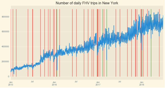
In our dataframe, we therefore have a “counts” column, a “is_holiday” column, and a “is_bad_weather” column. However, given we want to make predictions, we need to “anticipate” these dates as we would do for future predictions, we will therefore create two additional columns indicating that the next day is a holiday or that extreme weather is expected the next day :
weather = [datetime.datetime.strptime(date, "%Y-%m-%d") for date in ['2018-01-04', '2018-03-21','2017-03-14','2017-02-09','2016-01-23']]
holidays = [date for y in range(2015, 2019) for date, _ in sorted(holidays.US(years=y).items())]
df['is_holiday'] = np.where(df.index.isin(holidays), 1, 0)
df['bad_weather'] = np.where(df.index.isin(weather), 1, 0)
df['next_is_holiday'] = df.is_holiday.shift(-1)
df['next_bad_weather'] = df.bad_weather.shift(-1)
Choice of window size & Backtesting
When doing time series forecasting you might hear about backtesting. Backtesting is a procedure used during training which consists in splitting your data into chunks, in an incremental manner. At each iteration, a chunk is used as your training set. You then try to predict 1 or more values ahead of your chunk. Two approaches can be used, expanding and sliding windows:
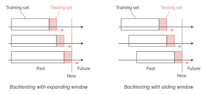
In our case study, the authors use samples consisting of 28-days sliding windows with step size equal to 1, used to predict the next value (1-step ahead forecast).
Logging and scaling
In the paper, the authors start by taking the log of the data to “ alleviate exponential effects”. They then within each window substract the first value of the window to remove the trend and train the network on fluctuations with regard to the first value of the window(eq(1)). Other approaches can also be thought of, such as substracting the first value and dividing by the first value (eq(2)):

Building the Dataset
Our dataset will be a generator yielding batches of sliding windows (each batch is the previous batch shifted of 1 value in the future). To follow the paper’s instructions, we will also substract, within each batch, the first value to all other values. Each batch is then split between 28-days samples and their 1-day targets.
def create_dataset(dataset, look_back=1, forecast_horizon=1, batch_size=1):
    batch_x, batch_y, batch_z = [], [], []
    for i in range(0, len(dataset)-look_back-forecast_horizon-batch_size+1, batch_size):
        for n in range(batch_size):
            x = dataset[['log_counts','next_is_holiday','next_bad_weather']].values[i+n:(i + n + look_back), :]
            offset = x[0, 0]
            y = dataset['log_counts'].values[i + n + look_back:i + n + look_back + forecast_horizon]
            batch_x.append(np.array(x).reshape(look_back, -1))
            batch_y.append(np.array(y))
            batch_z.append(np.array(offset))
        batch_x = np.array(batch_x)
        batch_y = np.array(batch_y)
        batch_z = np.array(batch_z)
        batch_x[:, :, 0] -= batch_z.reshape(-1, 1)
        batch_y -= batch_z.reshape(-1, 1)
        yield batch_x, batch_y, batch_z
        batch_x, batch_y, batch_z = [], [], []
Defining the model
We will use PyTorch to define our model. A simple reason for that is that we will use dropout during inference and that it is simple to implement in PyTorch. We will start by using a simple LSTM network as defined in the paper: 1 LSTM layer with 128 units, 1 LSTM layer with 32 units, and a fully connected layer with 1 output. Dropout is added after each layer.
— An aparté on Dropout Dropout can be seen as a way of doing Bayesian inference (though there is still a debate around this). Technically, dropout is the process used in neural networks consisting in randomly dropping units (along with their connections). The fact of randomly turning neurons on and off is roughly equivalent to performing a sampling of a Bernoulli distribution, and therefore “simulates” the mechanics of a Bayesian Neural Network (where weights are distributions, and not single values). Applying dropout is a bit like if we were “sampling” from the network. And if we repeat this process several times duting inference, we will get different predictions with which we can estimate a distribution and eventually, uncertainty ! To sum up:
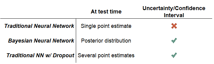
Let’s now define the model by adding dropout layers between each LSTM layer (notice how train is set to True so that Dropout is used during training and testing)
import torch
import torch.nn as nn
import torch.nn.functional as F
from torch.autograd import Variable

class Model(nn.Module):
    def __init__(self, config):
        super(Model, self).__init__()
        self.hidden_size = 128
        self.bi = 1
        self.lstm = nn.LSTM(config.get('features'),self.hidden_size,1,dropout=0.1,bidirectional=self.bi-1,batch_first=True)
        self.lstm2 = nn.LSTM(self.hidden_size,self.hidden_size // 4,1,dropout=0.1,bidirectional=self.bi-1,batch_first=True)
        self.dense = nn.Linear(self.hidden_size // 4, config.get('forecast_horizon'))
        self.loss_fn = nn.MSELoss()

    def forward(self, x, batch_size=100):
        hidden = self.init_hidden(batch_size))
        output, _ = self.lstm(x, hidden)
        output = F.dropout(output, p=0.5, training=True)
        state = self.init_hidden2(batch_size)
        output, state = self.lstm2(output, state)
        output = F.dropout(output, p=0.5, training=True)
        output = self.dense(state[0].squeeze(0))

        return output

    def init_hidden(self, batch_size):
        h0 = Variable(torch.zeros(self.bi, batch_size, self.hidden_size))
        c0 = Variable(torch.zeros(self.bi, batch_size, self.hidden_size))
        return h0, c0

    def init_hidden2(self, batch_size):
        h0 = Variable(torch.zeros(self.bi, batch_size, self.hidden_size//4))
        c0 = Variable(torch.zeros(self.bi, batch_size, self.hidden_size//4))
        return h0, c0

    def loss(self, pred, truth):
        return self.loss_fn(pred, truth)
Training
We train for 5 epochs, with an Adam optimizer and learning rate set to 0.001, and batch_size of 1.
batch_size = 1
forecast_horizon = 1
look_back = 28
model = Model(dict(features=3, forecast_horizon=1))
optimizer = torch.optim.Adam(model.parameters(), lr=0.001)
n_epochs = 5

model.train()
train_true_y = []
train_pred_y = []
for epoch in range(n_epochs):
    ep_loss = []
    for i, batch in enumerate(create_dataset(df[df.index<"2018"], look_back=look_back, forecast_horizon=1, batch_size=batch_size)):
        print("[{}{}] Epoch {}: loss={:0.4f}".format("-"*(20*i//(len(df[df.index<"2018"])//batch_size)), " "*(20-(20*i//(len(df[df.index<"2018"])//batch_size))),epoch, np.mean(ep_loss)), end="\r")
        try:
            batch = [torch.Tensor(x) for x in batch]
        except:
            break

        out = model.forward(batch[0].float(), batch_size)
        loss = model.loss(out, batch[1].float())
        if epoch == n_epochs - 1:
            train_true_y.append((batch[1] + batch[2]).detach().numpy().reshape(-1))
            train_pred_y.append((out + batch[2]).detach().numpy().reshape(-1))
        optimizer.zero_grad()
        loss.backward()
        optimizer.step()
        ep_loss.append(loss.item())
    print()
Results :
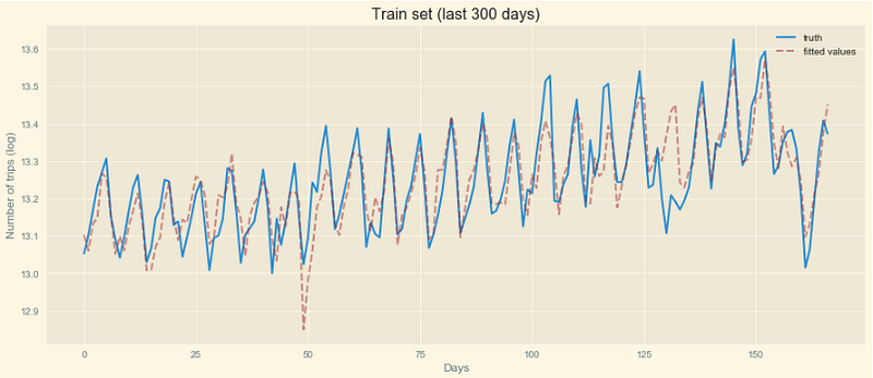
Testing — 1 day forecast horizon
One of the key interests of this paper is the estimation of uncertainty.
Specifically, stochastic dropouts are applied after each hidden layer, and the model output can be approximately viewed as a random sample generated from the posterior predictive distribution. As a result, the model uncertainty can be estimated by the sample variance of the model predictions in a few repetitions.
The idea behind this paper is therefore to run several times the model with random dropout, which will yield different output values. We can then compute the empirical mean and variance of our outputs to get confidence intervals for each time step !
n_repeats = 10
test_true_y = []
test_pred_y = []
for repeats in range(n_repeats):
    ep_loss = []
    preds = []
    for batch in create_dataset(df[df.index>="2018"], look_back=look_back, forecast_horizon=1, batch_size=1):
        try:
            batch = [torch.Tensor(x) for x in batch]
        except:
            break
        out = model.forward(batch[0].float(), batch_size=1)
        loss = model.loss(out, batch[1].float())
        ep_loss.append(loss.item())
        if repeats == 0:
            test_true_y.append((batch[1] + batch[2]).detach().numpy().reshape(-1))
        preds.append((out + batch[2]).detach().numpy().reshape(-1))
    print("{:0.4f}".format(100*np.mean(ep_loss)), end=", ")
    test_pred_y.append(preds)
test_true_y = np.array(test_true_y)
test_pred_y = np.array(test_pred_y)

mean = np.mean(test_pred_y, axis=0).reshape(-1)
std = np.std(test_pred_y, axis=0).reshape(-1)
lower = np.percentile(test_pred_y, 5, axis=0).reshape(-1)
upper = np.percentile(test_pred_y, 95, axis=0).reshape(-1)

fig, ax = plt.subplots(figsize=(15,6))
ax.plot(np.array(test_true_y).reshape(-1), label='truth')
ax.plot(mean, label='pred', c='brown', linestyle='--', alpha=0.5)
ax.fill_between([*range(len(test_true_y.reshape(-1)))], mean-2*std, mean+2*std, label='95%', color='brown', alpha=.3)
ax.fill_between([*range(len(test_true_y.reshape(-1)))], mean-3*std, mean+3*std, label='99%', color='orange', alpha=.4)
ax.set(title="Test set - 1 step ahead forecast", ylabel="Number of trips (scaled)", xlabel="Days", ylim=(12.7, 13.8))
ax.legend();
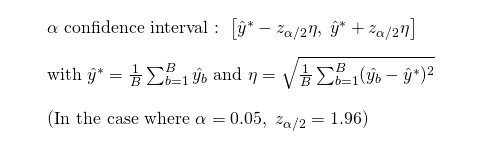
For each step, we predict 100 values. All values are different given we keep the dropout set. This allows us to simulate sampling from our network (in fact, Dropout is closely linked to Bayesian Neural Networks, given that by randomly disconnecting weights, it simulates a probability distribution). We take the average of these 100 values as our predicted mean, and the standard deviation of our 100 values which will be used for our confidence intervals. Assuming that our predictions are drawn from a normal distribution N(μ, σ²) — with a mean μ equal to our empirical mean and a standard deviation σ equal to our empirical standard error —, we can then estimate confidence intervals. In our case, it is given by :
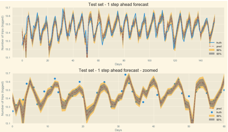
The prediction and the test curves seem to be quite close ! However, we need to find a metric to see how our model performs.
If we look at the empirical coverage of 95% predictive intervals (ie the number of true test values included in the predicted 95% confidence intervals), we obtain a value of 28.51%, far from the values obtained on the test set in the paper…When we take the 99% CI, this value goes up to 44% coverage. This is not a great result, but keep in mind our confidence interval is quite small given we only predict model uncertainty…
Testing — 7 days forecast horizon
Results on a single day forecast are not so good for a prediction model, and still we are not asking a lot to our model as we are asking for a very short prediction horizon. What if we trained our model to predict larger horizon forecasts ?
Conclusion
LSTMs show interesting perspectives for modelling time series due to their ability to capture long time dependencies, but should be used only for large datasets. Never expect your RNN to give good results on a 100-sample dataset ! The balance between the number of parameters in a neural network and the size of the data available is important to avoid overfitting. Nikolay Laptev, one of the authors of the Uber paper, concludes by saying that :
Classical models are best for: ○ Short or unrelated time-series ○ Known state of world
Neural Network is best for: ○ A lot of time-series ○ Long time-series ○ Hidden interactions ○ Explanation is not important